Carbon Inequality: Price Discovery and Market Dynamics in the Voluntary Carbon Market

WFE Research Working Paper No. 11. WFE Research Working Papers present work in progress by the author(s) and are published to receive feedback and stimulate debate. Comments on Research Working Papers are welcome and may be sent to the WFE Head of Research, [email protected].

Carbon inequality: price discovery and market dynamics in the voluntary carbon market¹ by Ying Liu²  November 19, 2025

Abstract

The voluntary carbon market (VCM) facilitates the trading of carbon credits, which represent verified emission reductions that firms may use to offset their carbon footprints by investing in sustainable projects. This study quantifies the determinants of carbon credit prices. It finds that prices are generally higher for nature-based projects than for technology-based ones and are significantly affected by credit age and total supply. A complementary machine learning analysis confirms these relationships, identifying past returns and prior credit inventory as two key drivers of price variation.

Moreover, carbon credits from advanced economies command a substantial premium, with average prices approximately 28% higher than those from emerging markets and developing economies. This disparity cannot be explained by credit characteristics or investor home bias; rather, it is closely linked to differences in governance quality across project jurisdictions, particularly the rule of law.

These findings highlight regional price inequalities and the need for improved pricing transparency.

Keywords: Voluntary carbon market, carbon credits, carbon offsets, price discovery

JEL classification: G12, G15, G18, O44, Q4

1 Introduction 

The voluntary carbon market (VCM) contributes to global climate change mitigation by providing entities with the option to offset their greenhouse gas emissions through the purchase of carbon credits. These credits, generated by projects that reduce or remove carbon emissions, offer a market-based mechanism for corporations and individuals to achieve their environmental objectives beyond regulatory mandates.³ As the urgency of addressing climate change intensifies, the voluntary carbon market has gained prominence as a complementary tool to compliance markets, broadening participation in decarbonization efforts. Nonetheless, the market remains highly fragmented, with disparities in pricing, credit quality, and regulatory oversight. Its effectiveness and scalability have been further constrained in recent years by growing scrutiny of credit integrity from NGOs and media, high-profile allegations of greenwashing, delays in guidance from initiatives such as the SBTi and ICVCM, and the absence of harmonized standards and transparency.⁴

Despite its potential, the voluntary carbon market faces challenges in ensuring fair pricing and market access for emerging and developing economies. Most carbon offset projects are based in these regions, where emission reduction costs are lower and climate finance is critical for sustainable development.⁵ However, emerging markets and developing economies often lack the financial resources needed for climate adaptation and mitigation.⁶ This issue has been a key topic in international climate negotiations, including COP29, where developing nations have called for fairer carbon market mechanisms and stronger financial support to bridge the climate finance gap. Ensuring that funds reach the communities and ecosystems they aim to support is essential for achieving the Paris Agreement’s climate goals.

Given these challenges, understanding the mechanisms that drive carbon credit pricing and the underlying causes of price disparities is essential for improving the efficiency, transparency, and fairness of the voluntary carbon market (VCM). This paper examines the key factors influencing price formation in the VCM, with particular attention to the persistent price gap between credits issued in advanced economies (AEs) and those from emerging market and developing economies (EMDEs). We analyse how project-level characteristics, market structure variables, and jurisdictional factors jointly contribute to these pricing differences. In doing so, we aim to inform both academic understanding and policy debates on how to design a more equitable carbon trading system. 

To conduct this analysis, we use transaction-level data from AlliedOffsets, a comprehensive database tracking the voluntary carbon market. The dataset covers carbon credit retirements from January 2017 to December 2024, with transaction records detailing credit prices, project characteristics, registry platforms, and transaction volumes.⁷ The data allow for a granular examination of price determinants. We complement traditional econometric techniques with machine learning methods, which enables us to cross-validate findings and identify robust patterns in the determinants of carbon credit prices. 

The first research question addresses the determinants of carbon credit prices, focusing on the roles of project characteristics, credit attributes, and market structures. We document that nature-based projects, especially Forestry & Land Use, command substantial premia over technology-based credits, with median prices about 67% above Renewable Energy. Vintage year matters, as older credits trade at discounts of 9% to 23%, reflecting buyers’ preference for recent vintages that are perceived to deliver more credible and immediate climate benefits. Larger project inventories are associated with lower subsequent returns, consistent with a supply–demand mechanism in which abundant available credits exert downward pressure on prices. In the panel analysis, recent price changes exhibit strong mean reversion, indicating that short-term deviations from fundamental value tend to correct over time. By contrast, past return volatility is positively priced, suggesting that buyers may associate higher volatility with market activity or speculative interest, which can temporarily support prices. Complementary machine learning analysis using ridge regression and LightGBM confirms these patterns and consistently identifies lagged return and lagged inventory as the two most influential predictors of near-term price movements. 

We also detect a clear seasonality in voluntary credit retirements, with peaks occurring in December each year. This mirrors the pattern observed in compliance carbon markets and is likely linked to corporate sustainability reporting cycles and year-end offset commitments, consistent with the findings of ESMA (2022) for regulated markets. 

The second research question examines the AE–EMDE price disparity. In the full sample, credits from EMDEs are priced, on average, at USD 4.98 compared to USD 6.90 for AEs, representing an average discount of around 28%. This gap remains sizeable in matched-pair comparisons that control for project type, age, registry, and inventory, with EMDE credits still trading at about USD 1.65 per tonne less than otherwise similar AE credits. We then test whether home bias, proxied by a buyer’s preference for credits originating in the same country or region, explains the observed AE–EMDE price disparity. If home bias were present, we would expect higher relative prices for credits purchased from a buyer’s own jurisdiction or nearby regions, since the buyers are mainly from advanced economies. 

However, incorporating buyer–project geographic proximity (same country, same continent, or distance) into our regressions does not yield a significant or robust effect. Instead, we find robust evidence that stronger governance, particularly rule of law and control of corruption as measured by the World Bank’s Worldwide Governance Indicators, is associated with higher credit prices. This pattern indicates that market participants place a premium on institutional credibility and legal certainty, consistent with evidence from global equity markets showing that governance quality shapes carbon-transition risk premia (Bolton and Kacperczyk, 2023), and with broader findings that stronger institutions lower transaction costs and enhance market integrity (Jarmuzek and Lybek, 2018; Wetterberg et al., 2025).

Overall, our analysis provides a detailed, transaction-level view of price formation and jurisdictional disparities in the VCM. The findings highlight the dual challenge of improving market efficiency while reducing inequities in access to capital for high-quality projects in EMDEs. By quantifying the influence of jurisdictional governance, market microstructure, and project attributes on credit prices, the results offer practical guidance for policymakers, registries, and investors aiming to strengthen the credibility and comparability of voluntary carbon markets.

Related Literature Research on voluntary carbon markets remains limited. Pedersen (2023) shows that allowing firms to use low-quality carbon offsets undermines the effectiveness of carbon pricing and green finance by distorting the true cost of emissions. The paper emphasizes that only high-quality offsets (i.e., with verified additionality and permanence) can preserve environmental integrity and prevent greenwashing in voluntary carbon markets. Kim et al. (2024) examine firm use of offsets and document that larger, institutionally held, net-zero-committed firms are more likely to use offsets; importantly, offsets are used intensively in low-emission industries and can increase after an exogenous ESG rating downgrade, consistent with strategic rather than purely impact-driven offsetting. Esenduran et al. (2024) analyse firms’ choices between buying offsets themselves versus inviting consumers to purchase add-on offsets, finding conditions under which consumer participation improves environmental outcomes and profitability by leveraging willingness to pay while reducing corporate outlays.

Policy-oriented analyses provide complementary insights into the governance and regulatory architecture of the voluntary carbon market. Reports by IOSCO (2023b) and World Bank (2023, 2024a) stress the need for robust integrity safeguards, transparent pricing, and credible verification frameworks to build market trust and effectiveness. These institutional considerations are central to understanding pricing dynamics in settings without statutory enforcement. 

A larger empirical literature focuses on compliance carbon markets, particularly the EU ETS. Green (2021) find that carbon pricing delivers modest annual emissions reductions (0–2%) and requires complementary measures, such as renewable mandates, to achieve deep decarbonization. Cludius et al. (2022) report no evidence that financial actors manipulate EUA prices through squeezing or cornering, while Quemin and Pahle (2023) caution against excessive speculation and advocate improved monitoring tools. Borri et al. (2024) document trading inefficiencies, with many firms trading only during surrender months and a subset engaging in excessive, profit-driven activity. Together, these studies underscore how market structure and participant behaviour influence efficiency and price formation in regulated settings. 

Within the compliance literature, several studies examine the firm-level effects of carbon pricing. Using plant-level data from California’s cap-and-trade programme, Bartram et al. (2022) show that financially constrained firms reduce emissions in regulated jurisdictions but shift output to unregulated states, illustrating regulatory spillovers. Bustamante and Zucchi (2024) develop a dynamic carbon management model, showing that carbon pricing reduces emissions but shifts firms’ green investment toward immediate abatement rather than long-term innovation. This reflects an intertemporal trade-off: abatement delivers quick reductions in expected carbon liabilities, whereas innovation has delayed and uncertain benefits. In the European context, Bolton et al. (2023) find that stock price reactions to EU ETS price changes depend on firms’ allowance positions, with permit shortfalls linked to negative returns. These studies highlight how compliance-market prices transmit through both regulatory and financial channels.

This paper contributes to the literature by analysing price formation in the voluntary carbon market, where prices are shaped not by compliance obligations but by buyer preferences, certification standards, and the credibility of host-country institutions. 

In contrast to compliance markets, VCM price dynamics emerge from voluntary participation and third-party verification. In this respect, our results also resonate with Bolton and Kacperczyk (2023), who document a global “carbon premium”—higher stock returns for high-emission firms, especially in countries with weaker institutions and greater fossil-fuel dependence. We find a parallel institutional channel in the VCM: stronger governance, particularly the rule of law, is associated with higher credit prices, which helps to explain persistent AE–EMDE price gaps even after controlling for project characteristics. 

This study contributes to the literature by providing the first transaction-level analysis of voluntary carbon credit pricing that links micro-level project attributes to macro-level governance factors. By comparing these patterns to established evidence from compliance markets, we offer new insights into how market design and institutional quality jointly shape carbon credit valuation in an unregulated environment. 

The paper is organized in the following way: Section 2 introduces the carbon markets, provides relevant background information, and offers an overview of the data. In Section 3, we analyse the factors influencing carbon credit pricing. Section 4 investigates the price differences between advanced economies and emerging and developing economies. Section 5 presents robustness checks to validate our findings. Finally, Section 6 summarizes the key insights and conclusions of the study. Supplementary tables and figures are provided in the Appendix.

2 Institutional Background and Data

2.1 Institutional background

The foundation of carbon markets can be traced back to the Kyoto Protocol, adopted in 1997 under the United Nations Framework Convention on Climate Change (UNFCCC) and formally implemented in 2005. The Kyoto Protocol introduced legally binding greenhouse gas (GHG) emission reduction targets for developed countries, marking one of the first major international efforts to combat climate change. 

To facilitate compliance with these targets, carbon markets were established as a market-based mechanism, assigning a value to GHG emissions and enabling both countries and firms to achieve their climate goals in a cost-effective manner. 

Carbon markets are broadly categorized into two types: compliance carbon markets (CCMs) and voluntary carbon markets (VCMs). These markets differ in their regulatory structures and in the nature of the carbon products traded. 

Compliance carbon markets, also referred to as Emission Trading Systems (ETSs), were formally established in 2005 as a result of the Kyoto Protocol. These markets operate under mandatory regulatory frameworks at the national, regional, or international level, requiring participants, primarily businesses and industries, to meet legally binding emission reduction targets. The key trading instrument within compliance markets is the carbon allowance, a government-issued permit that grants the holder the right to emit one metric ton of CO2 equivalent (tCO2e). The overall supply of allowances is typically capped by governments to create scarcity and drive emission reductions.⁸ The global compliance carbon market reached a record value of $948.75 billion (€881 billion) in 2023. The European Union’s Emissions Trading System (EU ETS) remained the dominant market, accounting for €770 billion, which represented 87% of the global market share (Twidale, 2024). 

In contrast to compliance markets, voluntary carbon markets function under a non-mandatory mechanism that allows firms, institutions, and individuals to offset their carbon footprints by purchasing carbon credits. These credits, sometimes referred to as carbon offsets, are generated by projects that either prevent GHG emissions (e.g., renewable energy or forest conservation projects) or actively remove CO2 from the atmosphere (e.g., reforestation or direct air capture initiatives).⁹ Each carbon credit represents a reduction or removal of one metric ton of CO2 equivalent (tCO2e). Unlike compliance markets, which are subject to government-imposed regulations, voluntary carbon markets function within self-regulated frameworks that rely on independent verification standards to ensure the integrity of carbon credits.¹⁰ 

The lifecycle of carbon credits follows a structured process that includes three main stages: project initiation, credit issuance and verification, and credit trading or retirement. 

The first stage, project initiation, begins with the development of a carbon project. A project developer is responsible for designing, implementing, and listing the project in an independent carbon registry. Registries set specific eligibility criteria and methodologies that projects must follow to ensure credibility. Before a project is approved, it undergoes a validation process by an independent validation and verification body, which assesses whether the project design meets the required standards. If the project passes validation, the registry certifies the project and approves a crediting period, which defines the time frame during which the project can generate and issue carbon credits. 

Once the project is operational, it enters the second stage, credit issuance and verification. During this phase, the project’s actual greenhouse gas reductions must be measured, reported, and verified (MRV). The emission reductions are compared against a baseline scenario, which estimates the emissions that would have occurred without the project. The project developer compiles this data into a monitoring report and submits it for verification by an accredited third party. If the verification confirms that the project has successfully reduced emissions, the carbon registry issues carbon credits based on the verified reductions. 

The final stage is credit trading or retirement. Once issued, carbon credits can be bought and sold in the secondary market by companies, institutions, and investors seeking to meet compliance obligations or engage in voluntary offsetting. Alternatively, organizations and individuals can retire carbon credits to compensate for their own emissions. Retiring a credit means permanently removing it from circulation so that it cannot be resold or reused. Carbon registries record all transactions and retirements to maintain transparency and prevent double counting. They also facilitate the transfer of credits between buyers and sellers, ensuring a smooth and reliable settlement system. 

The secondary market for carbon credits operates through over-the-counter (OTC) trading and organized exchanges. In the OTC market, transactions are conducted bilaterally through brokers or dealers, offering flexibility but providing limited transparency. According to (IOSCO, 2023b), most carbon credit transactions occur bilaterally or via intermediaries. In contrast, organized platforms provide standardized trading protocols, enhancing liquidity and price discovery.¹¹ 

Registries play a crucial role in ensuring the integrity, transparency, and credibility of carbon credits. They function as centralized databases, tracking the issuance, transfer, and retirement of carbon credits to prevent double counting and ensure that each credit represents a verified emission reduction or removal. Some of the largest and most widely recognized registries in the voluntary carbon market include Verra (Verified Carbon Standard — VCS), Gold Standard (GS), American Carbon Registry (ACR), and Climate Action Reserve (CAR). Together, these four registries accounted for approximately 94% of all carbon credits issued globally by the end of 2024 (Liu and Gurrola-Perez, 2025). 

Carbon projects vary in type and can be categorized into different sectors or scopes, each targeting a specific approach to emission reduction or removal. For example, the Voluntary Registry Offsets Database (VROD) groups carbon projects into nine major categories: Agriculture, Carbon Capture & Storage, Chemical Processes, Forestry & Land Use, Household & Community, Industrial & Commercial, Renewable Energy, Transportation, and Waste Management.¹² 

A carbon project may span several years, meaning the carbon credits it generates can be distributed across multiple years. Each credit is assigned a vintage year, which refers to the year in which the emission reduction or removal actually occurs (or is projected to occur in the future). In contrast, the issuance date is the point at which a carbon credit is formally recognized and made available for trading. This date is typically later than the vintage year, sometimes by several years, due to the validation, verification, and certification processes required to ensure the project’s legitimacy.¹³ Liu and Gurrola-Perez (2025) document that the average duration from the credit vintage year to the year of credit issuance is 2.45 years. 

Beyond their primary function of reducing carbon emissions, many carbon projects generate additional social, economic, and environmental benefits, commonly referred to as co-benefits. These can include job creation in local communities, biodiversity conservation, improved air and water quality, and public health improvements. Recognizing the broader impact of carbon projects, major carbon registries have introduced verification schemes to assess whether projects align with the UN Sustainable Development Goals (SDGs), further enhancing their transparency and credibility.

To further validate these co-benefits, many carbon projects seek certification under the Climate, Community & Biodiversity (CCB) Standards, developed by Verra. The CCB Standards assess a project’s social and environmental impact, certifying those that provide substantial benefits beyond carbon sequestration. Projects achieving Gold Level CCB certification demonstrate exceptional contributions to biodiversity, climate adaptation, and community well-being.

2.2 Data 

This study utilizes transaction-level data on carbon credits from AlliedOffsets, a comprehensive database tracking VCM transactions. The dataset includes detailed records of carbon credit trades, covering information on carbon projects, project developers, registries, credit purchasers, and carbon credit pricing.¹⁴ By using this granular dataset, we aim to analyse price discovery mechanisms within the voluntary carbon market and identify key factors that influence carbon credit pricing dynamics.

Our analysis covers the period from January 2017 to December 2024. This time frame ensures higher data reliability, as AlliedOffsets began incorporating actual market data in 2022, while earlier years (2017–2021) rely on adjusted estimates based on Ecosystem Marketplace sectoral price trends.¹⁵

Several filters are applied to the dataset. First, transactions marked as “cancellation”, which denote the administrative delisting of credits from a registry, are excluded. Credits with missing vintage years or where the vintage year exceeds the transaction year are also removed.¹⁶ Projects lacking sector classification or categorised as “Other” are excluded from the analysis. Projects with transactions observed in only one month over the entire sample period are also excluded to ensure meaningful price variation and return estimation. Lastly, only credits issued by the major registries — American Carbon Registry (ACR), Climate Action Reserve (CAR), Gold Standard (GSR), and Verra — are retained.

The refined dataset includes 259,967 retirement records originating from 2,207 projects. Each record provides information on the transaction date, estimated price, credit volume, vintage year of credit, and project ID. To enhance the scope of the analysis, this transaction data is merged with detailed project attributes, including registry affiliation, sector classification, geographic location, project founding year, and project co-benefits.

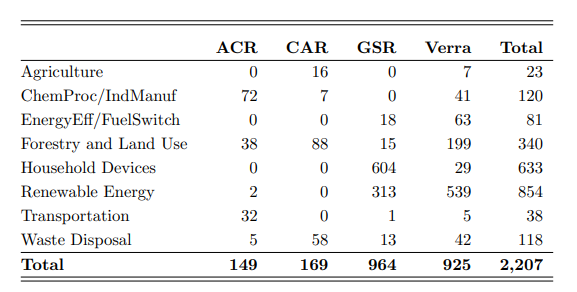
Table 1 provides an overview of the distribution of carbon projects by sector and registry. The dataset includes eight sectors: Agriculture, Chemical Processes/Industrial Manufacturing, Energy Efficiency/Fuel Switching, Forestry and Land Use, Household Devices, Renewable Energy, Transportation, and Waste Disposal. The registries demonstrate varying sectoral focuses. Verra accounts for the largest number of projects (925), with a significant emphasis on Renewable Energy (539 projects) and Forestry and Land Use (199 projects). Gold Standard predominantly focuses on Household Devices projects (604). Across sectors, Renewable Energy represents the largest category with 854 projects, followed by Household Devices (633) and Forestry and Land Use (340). In contrast, sectors such as Agriculture, Transportation, and Energy Efficiency/Fuel Switching feature fewer projects, indicating a more limited presence in these areas.

Table 1. Distribution of carbon projects by sector and registry 

This table summarizes the number of carbon projects by registry and sector. The column headers denote the registries, while the row headers represent project sectors. The “Total” column aggregates the number of projects within each sector, and the “Total” row summarizes the total projects across all registries. ChemProc/IndManuf refers to Chemical Processes/Industrial Manufacturing; EnergyEff/FuelSwitch refers to Energy Efficiency/Fuel Switching; CAR refers to Climate Action Reserve; GSR refers to Gold Standard; ACR refers to American Carbon Registry.

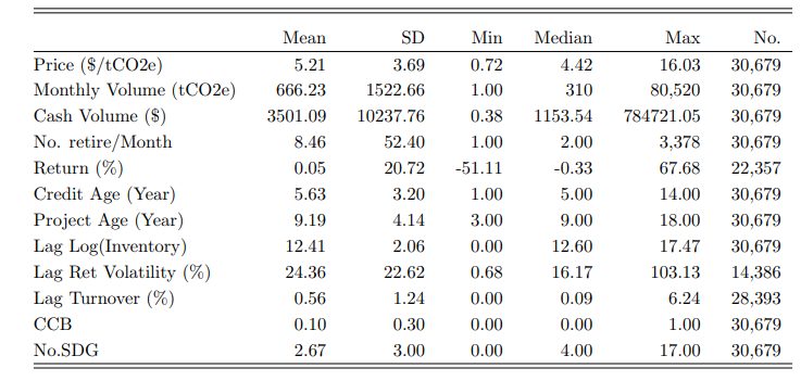
The trading of carbon credits is infrequent, with credits not being traded on a daily basis. To address this, the data is aggregated at a monthly frequency. We obtain 30,679 project-month observations. Specifically, monthly trading volume is calculated as the total volume of transactions within a month, while the monthly price is computed as the value-weighted average price, using transaction volumes as weights. Table 2 provides a summary of the key statistics for monthly carbon credit transactions.¹⁷

The average price of carbon credits is $5.21 per tCO2e, with a range of $0.72 to $16.03. Monthly trading volumes vary significantly, with an average of 666.23 tCO2e and a median of 310 tCO2e, though volumes range from as low as 1 tCO2e to a maximum of 80,520 tCO2e. The cash volume of monthly retirement is $ 3,501.09 per project. The average number of transactions per month, conditional on the existence of any transactions, is only 8.46, indicating the infrequent nature of carbon credit trading. This measure also exhibits substantial variability, with a minimum of one and a median of two transactions per month. These findings show that carbon credit transactions are irregular and mostly small in scale. 

Table 2 also reports additional summary statistics, which are utilized in the subsequent analysis.The return variable represents the monthly excess return on carbon credits, adjusted for the risk-free interest rate. To account for the infrequent nature of carbon credit trading, returns are calculated as scaled log returns, defined as the log price difference between two consecutive trades divided by the number of months between them.¹⁸ This approach mitigates distortions caused by irregular transaction intervals and improves consistency across projects. Despite a substantial reduction in observations due to these constraints, the average excess return is slightly positive at 0.05%, while the median is slightly negative at -0.33%, reflecting a wide dispersion in project-level performance. Credit Age, calculated as the volumeweighted average age of carbon credits at the time of transaction, is 5.63 years. This variable is calculated using transaction volume as the weight to account for the relative importance of larger trades. Project Age, defined as the duration between the year of project’s launch and the year of credit transaction, averages 9.19 years. Lag Return Volatility, which measures the standard deviation of the excess return over the past 12 months, has a mean value of 24.36%.¹⁹ This suggests substantial variability in the returns of carbon credits. Lag Log(Inventory) denotes the cumulative un-retired credits of previous month, and it is log transformed. The mean value of log(inventory) of previous month is 12.41, which translate to around 245,241.81 tCO2e. Lag Turnover is defined as the lagged value of project-level turnover, where turnover in month t is calculated as the ratio of the amount of retired credits to the lagged inventory (retired creditst/inventoryt−1 ), scaled by 100 to express it as a percentage. The variable exhibits considerable right skew, with a mean of 0.56% and a median of 0.09%, indicating that for most projects, monthly retirements constitute a small share of available inventory. Both CCB and No.SDG are dummy or discrete variables. CCB indicates whether a project has been verified under the Climate, Community & Biodiversity Standards, while No.SDG captures the number of United Nations Sustainable Development Goals (SDGs) a project aligns with. Only 10% of projects are verified by the CCB standards, and the average number of SDGs covered by a project is 2.67, with a median value of 4.²⁰

Table 2. Summary Statistics of Carbon Credit Transactions 

This table presents summary statistics for key variables related to carbon credit transactions. Price is the volume-weighted average price of carbon credits for a given project in a specific month. Monthly Volume refers to the total trading volume aggregated at the monthly level, while Cash Volume represents the value of the retired credits within a month. No. trans/Month indicates the number of retirement in a given month. Return is the excess return on carbon credits, calculated as the monthly return minus the risk-free interest rate. Credit Age is the volumeweighted average age of carbon credits at the time of transaction, using transaction volume as the weight. Project Age is the age of the project in years. Lag Return Volatility is the standard deviation of the excess return over the past 12 months. Lag Turnover is the ratio of retired credits over inventory from the previous month. CCB is a binary variable indicating whether the project is verified by the Climate, Community & Biodiversity (CCB) Standards. SDG is a binary variable that identifies whether a project aligns with the United Nations Sustainable Development Goals (SDGs). Lag Log(Inventory) represents the log-transformed accumulated un-retired carbon credits of a project from the previous month.

Next, we analyse the trends in the voluntary carbon market. Over time, the voluntary carbon market has experienced significant fluctuations. Liu and Gurrola-Perez (2025) report that while the issuance of carbon credits declined in 2022, credit retirements have shown a consistent upward trend over the years. Figure 1 illustrates the monthly average price and retirement volume of carbon credits in the sample. From 2017 to early 2021, prices were relatively stable, fluctuating between $2 and $5 per tCO2e. However, 2022 marked a dramatic price increase, peaking above $10 per tCO2e by mid-2022, followed by stabilization at levels significantly higher than the pre-2022 period.

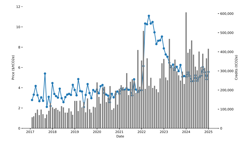
Figure 1. Monthly Price and Retirement volume of carbon credits This figure plots the monthly average price (blue line, left axis) and retirement volume (grey bar, right axis) of carbon credits from January 2017 to December 2024.

This price spike in early 2022 can be attributed to a combination of structural market factors and external geopolitical events. First, growing corporate commitments to net-zero targets increased demand for carbon credits, as companies sought to offset emissions in response to heightened ESG pressures. Second, shifts in market dynamics, including stricter scrutiny on credit quality and concerns over greenwashing, led buyers to prioritize high-integrity credits, reducing supply and driving up prices. 

Additionally, the Russia-Ukraine war in early 2022 likely played a role in the price surge by disrupting global energy markets. As fossil fuel prices soared due to supply chain disruptions and Western sanctions on Russian energy, prompting greater demand for carbon credits as a mitigation strategy. The geopolitical instability also reinforced corporate and investor interest in decarbonization, further accelerating purchases of offsets. Moreover, broader financial market uncertainty led some participants to view carbon credits as an alternative asset, increasing speculation and price volatility. and market uncertainty. By contrast, retirements slowed after early 2023, consistent with the downturn following integrity concerns, although monthly fluctuations have persisted into 2024.

By contrast, early 2023 marked a turning point. In January, a major media investigation raised concerns about the integrity of forest-based offsets from Verra, the largest crediting standard, reporting that a large share of rainforest credits were likely overstated or “worthless.”²¹ This triggered a sharp loss of market confidence, leading to a price correction and reduced retirement volumes as buyers reassessed credit quality and paused purchases. 

Retirement volumes displayed substantial variability, with notable spikes in 2022, during which monthly retirements frequently exceeded 400,000 tCO2e. These trends suggest that demand for carbon credits increased during periods of higher prices, as entities rushed to secure credits amid rising costs  and market uncertainty. By contrast, retirements slowed after early 2023, consistent with the downturn following integrity concerns, although monthly fluctuations have persisted into 2024.

3 Price Discovery 

As the voluntary carbon market continues to evolve, it has attracted increasing attention as a mechanism for channeling finance toward carbon offset projects globally. Despite growing project issuance and broader stakeholder engagement, overall transaction volumes remain limited, and liquidity in the secondary market is thin. These structural constraints, combined with a lack of price transparency, pose challenges for understanding market behaviour and pricing dynamics. In this section, we begin with a univariate analysis to assess whether specific characteristics, such as project sector, affect credit pricing. We then expand the analysis using a multi-factor framework to examine how various attributes jointly influence price variation in the voluntary carbon market. Next, we apply machine learning methods to evaluate the robustness of our results and to identify the most influential predictors of carbon credit returns. Finally, we investigate seasonal patterns in credit retirements, drawing parallels with compliance carbon markets to assess cyclical drivers of demand.

3.1 Univariate analysis 

To build initial intuition about the determinants of carbon credit pricing, we begin with a univariate analysis examining individual project characteristics, such as sector classification. This approach provides a descriptive overview of how credit prices vary across different categories, helping to identify broad patterns and potential drivers of price dispersion. While limited in its ability to capture interactions or confounding effects, this step serves as a useful foundation for the more comprehensive multivariate analysis that follows.

Different project sectors vary in environmental impact, risk profiles, and market demand, all of which can significantly shape pricing dynamics. Prices may differ across sectors due to variations in project implementation costs, for example, nature-based solutions like afforestation or carbon sequestration often require extensive land management and long-term monitoring, whereas industrial projects may involve lower upfront costs but face regulatory uncertainties. Risk is another key factor; forestry projects, for example, are exposed to threats like wildfires and illegal deforestation, raising concerns about the permanence of carbon sequestration, while renewable energy projects typically have more predictable emission reductions. Additionally, market demand for carbon credits differs by sector, as buyers may prefer credits from projects that align with corporate sustainability goals or provide co-benefits such as biodiversity conservation. These differences suggest that the project sector significantly influences pricing dynamics, making it essential to analyse how specific sectoral characteristics affect carbon credit valuation.

Table 3 presents key statistics for carbon credit transactions, categorized by project sector. These statistics include the volume-weighted average price, average monthly trading volume, credit age, project age, number of retirements per month, and co-benefits such as CCB verification and number of UN SDG. All values reflect the mean characteristics of projects within each sector, offering insights into sector-specific pricing trends.

Table 3. Summary Statistics of Carbon Credits by Project Sector 

This table presents the volume-weighted average price, monthly trading volume, credit age, project age, and number of retirements per month. The volume-weighted average price is calculated using trading volume as weights. All measures are averages of projects within the same sector. Last column reports the number of observations.

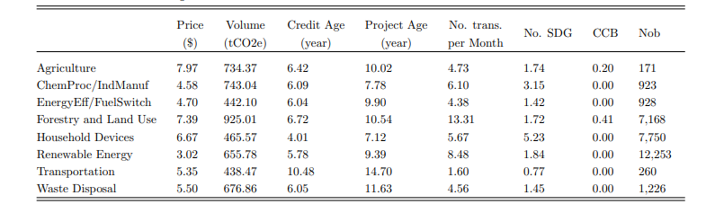
There exists significant variations in the characteristics of carbon credit transactions across different project sectors. Agriculture projects achieve the highest average price of $7.97, followed by Forestry and Land Use project of $7.39, suggesting that nature-based projects are generally valued more highly and perceived as more attractive to investors. Conversely, Renewable Energy projects report the lowest average price at $3.02, largely because of concerns about additionality and weaker “integrity” relative to nature-based credits.²² In terms of trading volumes, Forestry and Land Use projects exhibit the largest average monthly volume (925.01 tCO2e), while Transportation projects report the smallest (438.47 tCO2e). Credit age ranges from 4.01 years in Household Devices to 10.48 years in Transportation, indicating differing levels of maturity among credits. Similarly, project age spans from the relatively younger Household Devices projects (7.12 years) to the much older Transportation projects (14.70 years). 

Projects also differ in their sustainable development contributions: Household Devices projects report the highest average number of associated SDGs (5.23), while Transportation projects score the lowest (0.77).²³ In terms of co-benefit certification, 41% of Forestry and Land Use projects are CCB-certified, the highest across all sectors, whereas most other sectors report negligible or zero CCB certification. In summary, nature-based projects like Agriculture and Forestry and Land Use achieve higher prices and display robust trading activity, particularly Forestry and Land Use projects, which dominate in trading volume and transaction frequency. In contrast, Transportation projects experience lower transaction volumes and are characterized by older project and credit ages, suggesting lower market dynamics in this sector. 

To better understand the price distribution across different project sectors, we plot the prices of carbon credits by sector. Figure A1 illustrates the distribution of carbon credit prices for each project sector. Forestry and Land Use projects exhibit the widest price range, with a maximum price of approximately $16/tCO2e, a median around $5/tCO2e, and a mean of $7.39/tCO2e. This sector also shows a notable disparity between the mean and median values, indicating that a subset of transactions is associated with significantly higher prices. This price variation can be attributed to fluctuating market demand; Forest Trends’ Ecosystem Marketplace (2023) highlight that nature-based projects, particularly forestry and land use initiatives, commanded higher prices in 2021 and 2022 due to strong investor demand. 

However, in 2023, demand declined following high-profile media scrutiny over the accuracy of estimated emissions reductions from these projects, leading to greater price dispersion as market confidence shifted (Forest Trends’ Ecosystem Marketplace, 2024). In contrast, Renewable Energy projects have the lowest prices and the narrowest distribution, with both the median and mean around $3/tCO2e and maximum prices near $8/tCO2e. Sectors such as Energy Efficiency/Fuel Switching, Transportation, Household Devices, and Waste Disposal display similar price distributions, with medians clustering around $5/tCO2e. Overall, Forestry and Land Use projects exhibit the highest price variability, while sectors like Chemical Processes/Industrial Manufacturing and Renewable Energy show relatively narrow price distributions.

The univariate analysis offers key insights into how project sectors influence carbon credit pricing. Sectors such as Agriculture and Forestry and Land Use tend to have higher prices, likely due to their perceived environmental benefits and strong market demand, while Renewable Energy projects consistently trade at lower prices, reflecting differences in market valuation.

3.2 Multivariate analysis 

Building on the insights from the univariate analysis, this section takes a deeper look at the factors influencing carbon credit pricing using a multivariate approach. While the univariate analysis revealed significant differences across project sectors and registries, these factors do not operate in isolation. Instead, pricing dynamics result from the combined effects of project characteristics, market conditions, and other structural factors. By applying multivariate regression models, this analysis aims to quantify the relative contributions of these factors, offering a more comprehensive understanding of the drivers behind price variation in the voluntary carbon market. Given the relatively low trading frequency of carbon credits, the analysis is conducted on a monthly basis. For each project, we calculate the monthly volume-weighted average price and derive the corresponding monthly return. The regression model is specified as follows:

The dependent variable, Returni,t, represents the excess return of carbon project i in month t, calculated relative to the risk-free rate.²⁴ The vector of independent variables, Xi,t−1, includes several factors expected to influence carbon credit returns. Among them, credit age (Credit Agei,t) and project age (Project Agei,t) are particularly important. Older credits may decline in value due to changing market standards or evolving buyer preferences, while more mature projects may gain credibility, allowing them to command higher returns. 

The lagged return (Returni,t−1) captures potential momentum or mean-reversion effects by reflecting how past price movements influence investor expectations and future pricing behaviour. Lagged carbon credit inventory (Log(Inventory)i,t−1 ) measures the cumulative volume of unretired credits from prior periods, serving as a proxy for supply-side dynamics. A higher inventory level may indicate market oversupply, exerting downward pressure on prices, while lower inventory levels suggest scarcity, potentially driving prices upward due to increased competition among buyers. This variable accounts for the influence of market supply on credit returns. 

Lagged turnover (Turnoveri,t−1) is included to capture liquidity dynamics at the project level. Turnover is defined as the ratio of monthly retired credits to the lagged inventory, scaled by 100, and reflects the proportion of available supply that is transacted in a given month.²⁵ A higher turnover rate may indicate stronger market interest and better liquidity, potentially attracting more buyers and supporting higher returns. Conversely, low turnover could signal illiquidity, weak demand, or disinterest in the credit, all of which may depress returns. 

To assess the role of co-benefits, the variable CCBi,t indicates whether a project is certified under the Climate, Community & Biodiversity (CCB) Standards (1 if verified, 0 otherwise), reflecting its commitment to both environmental and social benefits. Similarly, No.SDGi,t denotes the number of United Nations Sustainable Development Goals (SDGs) the project aligns with, serving as a measure of broader sustainability contributions. 

Risk is captured through lagged return volatility (Volatilityi,t−1 ), computed as the standard deviation of returns over the previous 12 months.²⁶ Higher past volatility may indicate increased market uncertainty, prompting investors to adjust their required returns. This variable helps evaluate how historical fluctuations and perceived risk influence carbon credit pricing. To ensure robust analysis, all continuous variables except CCBi,t, and No.SDGi,t are winsorized at the 2.5th and 97.5th percentiles, mitigating the influence of outliers.

We include year-month, registry, and sector fixed effects to control for systematic differences and external influences on carbon credit prices. Year-month fixed effects account for time-specific shocks, trends, and seasonal variations, while registry fixed effects capture differences in verification standards, market acceptance, and institutional credibility. Sector fixed effects address pricing disparities across project types, reflecting variations in demand and regulatory contexts. These controls help isolate the impact of project-specific factors on returns. To ensure robust inference, standard errors are clustered at both the project and year-month levels.

Table 4. Multivariate Analysis Results 

This table reports the regression results for Equation (1). Column (1) excludes registry fixed effects, while Column (2) excludes project sector fixed effects. Column (3) includes both registry and project sector fixed effects. Column (4) further incorporates lagged return volatility as an explanatory variable. All models include year-month fixed effects. Standard errors are clustered at both the project and year-month levels. Statistical significance is denoted by * p<0.10, ** p<0.05 , *** p<0.01 

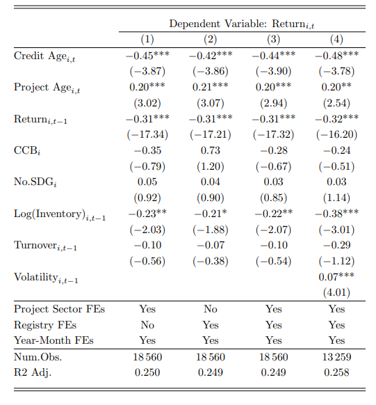
Table 4 presents the regression results analysing the determinants of monthly excess returns on carbon credits. All four models include year-month fixed effects. Model (1) includes project sector fixed effects but excludes registry fixed effects. Model (2) includes registry fixed effects while omitting sector controls. Model (3) incorporates both registry and project sector fixed effects. Model (4) adds lagged return volatility to the specification while retaining all fixed effects. Across all specifications, credit age exhibits a consistently negative and significant relationship with returns, suggesting that older credits, potentially perceived as outdated or of lower environmental integrity, are associated with lower performance. In contrast, project age is positively and significantly associated with returns, indicating that more established projects may benefit from increased credibility and buyer confidence.

The coefficient on lagged return is negative and highly significant in all models, providing strong evidence of mean reversion in carbon credit pricing. Projects that experienced higher returns in the previous month tend to see lower returns in the following month, a dynamic that may reflect temporary price adjustments or liquidity effects. The log of lagged inventory also shows a negative and significant relationship with returns, especially in Model (4), where its coefficient increases in magnitude and statistical significance. This result supports the view that oversupply of credits depresses future returns, highlighting the importance of inventory management in credit valuation.

CCB certification shows no significant relationship with returns across all specifications. This finding suggests that, after accounting for sector and registry differences, CCB certification does not command a return premium, potentially due to market saturation in sectors where CCB is prevalent or diminishing marginal valuation of co-benefits. The number of SDG-related claims is positively signed but statistically insignificant in all models, implying that SDG alignment may not directly translate into pricing advantages within the observed sample.

Lagged turnover, which is calculated as the proportion of inventory retired in the prior month, enters all models with a negative but statistically insignificant coefficient. While higher turnover may reflect past liquidity, its lack of significance suggests that recent trading activity does not predict future returns once other supply-side and project characteristics are controlled for.

Lagged return volatility (Volatilityi,t) is included as an explanatory variable in Model (4) to capture the influence of recent market uncertainty on returns. The coefficient is positive and statistically significant, suggesting that projects with greater past price fluctuations tend to offer higher future returns. This pattern aligns with the risk-return trade-off, where investors require additional compensation for bearing higher historical volatility.

Comparing Models (1) to (3), we find that the inclusion of registry and project sector fixed effects does not materially improve model fit, as reflected in nearly identical adjusted R2 values. This suggests that systematic return variation across registries or sectors is limited after controlling for key projectlevel fundamentals. In other words, observable attributes such as credit age, project age, and inventory dynamics play a much stronger role in explaining monthly excess returns than registry affiliation or project sector categorization. The consistency of results across these model specifications reinforces the reliability of the findings and underscores the role of both observable characteristics and structural market features in shaping carbon credit returns.

Overall, the findings suggest that carbon credit returns are influenced by a combination of project specific characteristics, market conditions, and institutional factors. Credit age is consistently associated with lower returns, likely reflecting declining market value for older credits, while project age is positively linked to performance, possibly due to enhanced credibility or operational maturity. Evidence of mean reversion is strong, and higher inventory levels are associated with lower returns, highlighting the role of supply dynamics. Certification effects appear limited: CCB verification does not exhibit a significant return premium once sector and registry factors are controlled for, and the number of SDG-related claims is also statistically insignificant, indicating that co-benefit signals may not be directly priced. Lagged return volatility is positively related to returns, consistent with risk-based pricing, though its statistical significance emerges only when included explicitly. Fixed effects for registries show no significant differences relative to Verra, while sectoral results indicate that Household Device and Waste Disposal projects underperform relative to Forestry and Land Use, with other sectors showing no clear return differentials (see table A1).

3.3 Machine learning analysis: robustness and variable importance 

To further explore the determinants of carbon credit returns and to complement the linear regression results in Section 3.2, we introduce two machine learning approaches that accommodate flexible, potentially nonlinear relationships among predictors. These models serve two main purposes: (i) to provide robustness checks on the explanatory power of selected variables, and (ii) to assess the relative importance of features across different frameworks.

Two representative machine learning methods are employed: Ridge regression, a linear model with regularization, and Light Gradient Boosting Machine (LightGBM), a flexible nonlinear model based on decision trees. Ridge regression extends the familiar linear regression model by adding a penalty term to prevent the estimated coefficients from becoming too large. This technique is particularly useful when many explanatory variables are correlated with each other, which often leads to unstable and unreliable estimates in ordinary least squares (OLS). By slightly shrinking the size of each coefficient, Ridge regression reduces overfitting and improves the model’s ability to generalize to new data, while still keeping all variables in the model. This makes Ridge especially helpful in settings where many potentially relevant variables are included, as is often the case in asset pricing applications (Gu et al., 2020).

In contrast to linear models, LightGBM is a machine learning approach based on decision trees. A decision tree works by repeatedly splitting the dataset into groups based on the values of predictor variables, aiming to isolate subsets of observations that behave similarly. At each split, the tree selects a variable and a threshold to best separate the remaining data, forming a branching structure of rules. The prediction is then made by averaging the outcome within each resulting group. By combining many such trees, LightGBM builds a powerful ensemble model that can flexibly capture nonlinearities, interactions, and threshold effects that are difficult to model with traditional linear regressions. This flexibility makes it especially effective in financial applications where variable relationships may not follow simple linear patterns (Ke et al., 2017).

To empirically assess the role of different feature groups, four model specifications are constructed based on the hypotheses discussed in Section 3.2. Model 1 includes all variables used in the baseline regression (1), covering numerical features such as lagged return and project characteristics, as well as categorical features such as registry and project sector dummies.²⁷ Model 2 adds lagged volatility(Volatilityi,t−1 ) to this set. Due to substantial missingness in volatility-related data, it is evaluated separately from Model 1 to preserve sample size.

Model 3 extends Model 1 by incorporating three additional macro-financial variables: the lagged excess returns of the S&P 500 index, crude oil, and the Climate Policy Uncertainty (CPU) index, along with interaction terms between these macro variables and the numerical features.²⁸ These macro variables are included to capture broader market trends, energy price shocks, and shifts in climate-related policy sentiment, all of which may influence investor behaviour and carbon credit returns.²⁹ Model 4 further augments Model 3 by adding lagged volatility and its interactions with the macro variables.

To ensure robustness and account for possible changes in model performance over time, a rollingwindow framework is used. The data is split into a series of consecutive, non-overlapping time blocks. In each block, the first 70% of observations form the training set, which is used to teach the model how to link predictors to returns. The next 15% is the validation set, which is used to try out different model settings and choose the ones that work best, helping to avoid overfitting to the training period. The final 15% is the test set, which is used to check how well the model performs on new, unseen data. After one block is evaluated, the whole window shifts forward by the length of the validation set, and the process repeats. This step-by-step approach reduces the chance of tailoring the model too closely to a particular period and helps detect changes in which features matter most, which is particularly important in fast-changing, policy-driven carbon markets. 

Table 5. Out-of-Sample Predictive Performance of Ridge and LightGBM Models 

This table reports the out-of-sample R2 and root mean squared error (RMSE) for Ridge regression and LightGBM across four model specifications. Model definitions are described in Section 3.2. The R2 values are computed using the corresponding test sets in the rolling window framework.

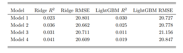
Model performance is reported in Table 5, using two complementary metrics: the out-of-sample R2 and the root mean squared error (RMSE). The R2 measures the proportion of variation in returns explained by the model, while the RMSE captures the average magnitude of prediction errors in the same units as the dependent variable, with lower values indicating greater accuracy. Ridge regression achieves its highest R2 and lowest RMSE in Model 4, which incorporates the most comprehensive set of predictors, including macroeconomic variables and lagged volatility. LightGBM, by contrast, attains its best performance in Model 1, which contains the smallest set of features. This difference reflects the way the two approaches work: Ridge regression handles a large number of predictors more steadily by keeping individual variable effects small and balanced, while LightGBM can sometimes lose accuracy when too many variables are included but is very effective at finding complex patterns and variable interactions when working with a more focused set of inputs.

Understanding which variables contribute most to predictive performance is essential for interpreting model outputs and linking statistical results to economic mechanisms. To this end, feature importance is examined for the best-performing specifications identified in Table 5: Model 4 of Ridge regression and Model 1 of LightGBM. The top 10 features from each are shown in Figure 2, where the Ridge plot reflects standardized coefficient magnitudes (with sign preserved) and the LightGBM plot shows normalized split-based importance scores.

Panel (a) of Figure 2 displays the top ten features from Ridge regression (Model 4), ranked by the absolute magnitude of their standardized coefficients while retaining their signs to indicate direction of effect. Key predictors include Lag Return, Lag Inventory, and Lag Volatility, alongside several interaction terms between macroeconomic variables and numerical features (e.g., Lag S&P 500 Return × Lag Return). Positive coefficients suggest that increases in these predictors are associated with higher expected returns, whereas negative coefficients imply the opposite. Notably, Lag Return emerges as the single most important feature, with a negative sign—consistent with the findings in Section 3.2—indicating a short-term reversal pattern in carbon credit returns. The second most important predictor, the interaction term Lag Oil Return × Lag Return, carries a positive sign, suggesting that the impact of recent carbon credit returns on future performance becomes more favorable when crude oil prices have also risen, potentially reflecting spillover effects from broader energy market dynamics. 

Panel (b) presents the top ten features from LightGBM (Model 1 ), ranked by normalized split frequency and gain across all trees in the ensemble.The most important predictor, Lag Return, reflects short-term momentum or reversal patterns; its prominence indicates that recent price movements remain a strong driver of near-term carbon credit returns. The second-ranked feature, Lag Inventory, proxies for market liquidity by capturing the size of available sell-side volume, with higher inventory potentially signaling greater supply pressure and influencing returns accordingly. 

Despite the differences in methodology, both Ridge regression and LightGBM consistently identify Lag Return and Lag Inventory as key predictors, reinforcing the central role of short-term price dynamics and market liquidity in shaping carbon credit returns. This convergence across a linear and a nonlinear framework suggests that these factors are robust drivers of return variation, regardless of model structure. Beyond this common ground, the two approaches diverge in the additional variables they emphasize: Ridge highlights macro–market interaction terms, reflecting its ability to extract stable linear effects from a broad predictor set, whereas LightGBM assigns greater importance to certain project-level characteristics, indicating that nonlinear models may be better suited to uncover conditional or threshold effects tied to project maturity, credit issuance patterns, and varying market environments. 

In summary, the machine learning analysis identifies Lag Return as the most influential determinant of carbon credit prices across both frameworks, consistent with short-term reversal dynamics documented in Section 3.2. This finding suggests that recent price movements exert a persistent, statistically significant influence on near-term returns. The second most important feature, Lag Inventory, measured as the lagged value of unretired credits, indicates that liquidity conditions and supply-side imbalances materially affect price formation. Beyond these core drivers, the Ridge model highlights the relevance of macroeconomic variables, particularly their interactions with Lag Return and Lag Inventory, implying that the influence of technical and liquidity factors is conditional on broader market conditions such as equity and energy price movements. While overall predictive power remains modest, the complementary perspectives of a linear regularized model and a nonlinear tree-based method, combined with a rolling window evaluation, provide a temporally robust and multifaceted understanding of the determinants of carbon credit returns.

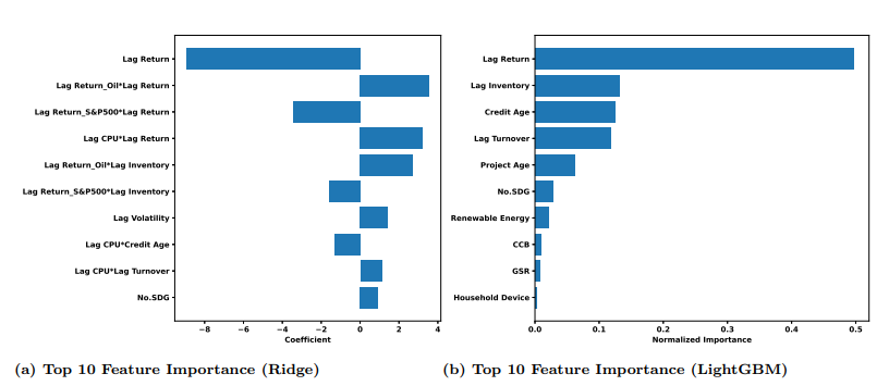
Figure 2. Comparison of Feature Importance from Ridge and LightGBM Models Panel (a) reports the top 10 features from Ridge regression (Model 4 ), where importance is measured by the absolute magnitude of standardized coefficients, preserving the sign to indicate direction of effect. Panel (b) reports the top 10 features from LightGBM (Model 1), where importance is measured by the normalized frequency and gain from feature splits across all trees.

3.4 Retirement seasonality 

Figure 1 illustrates the monthly retirement volumes of carbon credits, revealing a clear seasonal pattern. Retirements tend to peak at the beginning and end of the year, while mid-year months show relatively lower activity. This section further explores the monthly distribution of retirement volumes to understand these fluctuations. 

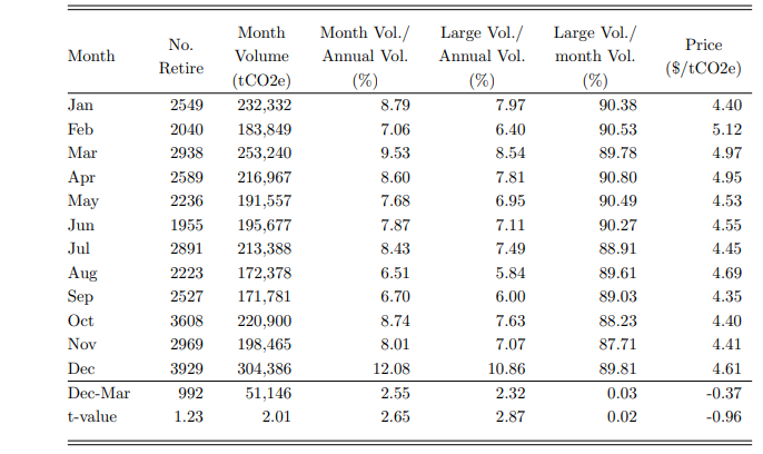
To analyse this pattern, we compute key retirement activity metrics for each month, including the average number of retirements, total monthly retirement volume, and each month’s share of the annual retirement volume. Table 6 summarizes these measures, consistently identifying December as the peak month. The average number of retirements in December is 3,929, significantly exceeding October, the second-highest month, with 3,608 retirements. December also leads in total retirement volume, reaching 304,386 tCO2e, followed by March at 253,240 tCO2e. On average, December accounts for 12.08% of the annual retirement volume, with March following at 9.53%. These findings align with previous studies, including Yadav (2024) and BloombergNEF (2024), which report a significant surge in carbon offset retirements in December 2023, reinforcing the trend of increased year-end activity in the voluntary carbon market. 

To formally assess whether December’s retirements are significantly higher than other months, we conduct a paired t-test comparing December and March, the second most active month, for each year. The last two rows of Table 6 present the mean differences between these months, along with their corresponding t-values. The results confirm that December’s retirement volume and share of annual retirements are significantly higher than those of March, establishing December as the peak period for carbon credit retirements. 

This pattern reflects practices commonly observed in compliance carbon markets, where December expiry futures contracts for the following (front) year are the most actively traded. This activity aligns with the lifecycle of emission allowances, which must be surrendered by April 30 each year (ESMA (2022)). A similar trend is evident in carbon offset futures, as illustrated in Figure A2. Decembermatured contracts for three different types of futures (C-GEO, GEO, and N-GEO) consistently exhibit the highest trading volumes, indicating a pronounced end-of-year demand surge across both compliance and voluntary carbon markets. 

A possible explanation from studies of compliance carbon markets is that companies are required to surrender CO2 emissions allowances by April each year, leading to increased trading activity in December EUA futures. In the voluntary carbon market, we observe a similarly pronounced spike in December retirement volume. Although our dataset does not directly identify retirement beneficiaries, we use retirements exceeding 100 tCO2e as a proxy for corporate involvement, as large-scale retirements are more likely to reflect institutional activity. Table 6 shows that December accounts for the highest share of annual large-scale retirements (10.86%), suggesting heightened engagement from corporate buyers during this month, potentially due to fiscal-year-end reporting or ESG disclosure cycles. However, the share of large retirements relative to total monthly volume in December (89.81%) is comparable to other months and does not deviate significantly from the average, implying that while absolute corporate retirement volume increases, the composition of retirement sizes remains relatively stable across months. This distinction suggests that corporate participation intensifies in December, but not disproportionately relative to smaller actors. 

Overall, the analysis in this section shows that price formation in the voluntary carbon market is shaped by a combination of project fundamentals, supply dynamics, and short-term market conditions. Older credits tend to trade at a discount, while more established projects and lower inventories support higher returns. The evidence of mean reversion in recent price changes, reinforced by both linear and nonlinear models, suggests that temporary imbalances in demand and supply are quickly corrected. Machine learning methods confirm the central role of lagged returns and inventory in explaining variation, while also highlighting conditional effects linked to macroeconomic factors and project characteristics. Seasonal peaks in retirements, concentrated in December, indicate that cyclical reporting and disclosure practices can generate predictable demand surges. Together, these findings point to a market where both structural attributes and temporal patterns matter for price discovery, offering insights for market participants and policymakers seeking to enhance transparency and efficiency.

Table 6. Carbon credit retirement activities by month 

This table reports the retirement activities by month. For each year from 2017 to 2024, we first calculate the value of each measure by each month, then we calculate the mean value of each measure across years for each month. No. Retire refers to the number of retirement of each month. Month volume is the aggregate credits retired of each month. Month Vol./Annual Vol. is the percentage of month volume over total retirement volume of a year. Large Vol./Annual Vol. is the percentage of retirement volume whose retirement is larger than 100 tCO2e over annual retirement volume. Large Vol./month Vol. refers to the percentage of aggregate retirement volume whose retirement is larger than 100 tCO2e over monthly retirement volume. Price refers to the value-weighted average price of each month. The last two rows reports the mean value and t-value of difference of each measure between December and March of a year.

4 Price Disparity 

Carbon credit projects are distributed globally, yet they are heavily concentrated in emerging market and developing economies (EMDE). Among the 2,204 projects analyzed in this study, 1,883 originate from EMDEs (see Table 7).³⁰ This dominance is consistent with Liu and Gurrola-Perez (2025), who report that EMDEs account for approximately 75% of total issuance in the voluntary carbon market. This highlights the important role these economies play in global climate mitigation efforts.

Despite this substantial contribution, EMDEs face persistent financing constraints. Although the COP29 summit set a target of $300 billion per year in climate finance for developing countries by 2035, many experts argue this is insufficient to meet decarbonization goals.³¹ Limited access to capital not only restricts project development but may also influence the market valuation of credits. If carbon credits from EMDEs are systematically undervalued relative to those from advanced economies (AE), this could exacerbate global inequality in climate finance and hinder progress toward shared environmental targets.

This section investigates whether such a pricing gap exists between AE and EMDE credits and seeks to identify its underlying drivers. Understanding this disparity is crucial for fostering a fair and efficient global carbon market that rewards climate outcomes regardless of geographic origin.

4.1 Price gap 

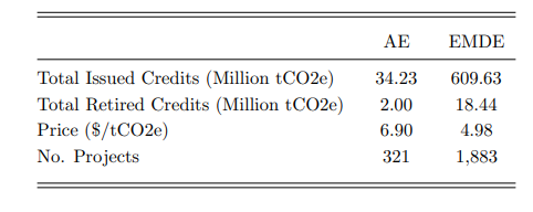
Table 7 presents key statistics by country group. Projects in EMDEs have issued a total of 609.63 million tCO2e, which is nearly 17 times more than the 34.23 million tCO2e issued in AEs. Similarly, retired volumes from EMDE projects total 18.44 million tCO2e, compared to just 2.00 million in AEs.

Interestingly, despite their lower issuance, advanced economies show a higher retirement rate (5.84%) than EMDEs (3.02%), suggesting relatively stronger demand. This is also evident in prices: the valueweighted average price of AE credits is USD 6.90 per tCO2e, compared to USD 4.98 for EMDEs. The EMDE average is also below the sample-wide average of USD 5.21 (Table 2).

Table 7. Statistics of carbon credits by project country 

This table reports the statistics of carbon credits grouped by project country. AE refers to Advanced Economies, EMDE refers to Emerging Market and Developed Economies. Total Issued (Retired) Credits are the aggregate quantity of carbon credits issued (retired) by projects of each group of country. Price refer to the value-weighted average price of each group, using retirement volume as weight. Value is the aggregate value of retired credits calculated as price times credit quantity. The sample spans from January 2017 to December 2024 and includes only carbon credits with available pricing data.

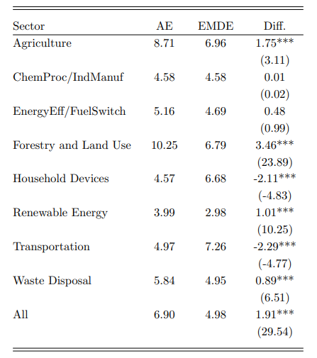
To examine pricing across different project types, Table 8 compares sector-level average prices between AE and EMDE projects. In most sectors, AE-based credits achieve higher prices. For example, Forestry and Land Use projects in AEs average $10.25 per tCO2e, compared to $6.79 in EMDEs. Agricultural projects also show a difference: $8.71 in AEs versus $6.96 in EMDEs. In contrast, EMDE credits in the Household Devices and Transportation sectors command higher prices than their AE counterparts. This variation suggests that sectoral composition and region-specific factors may influence observed pricing patterns.

Table 8. Average carbon credit price by project sector and country group 

This table reports the average price (in $/tCO2e) of carbon credits by project sector and by country group—Advanced Economies (AE) versus Emerging Market and Developing Economies (EMDE). The sample covers the period from January 2017 to December 2024 and includes only transactions with available pricing data. ChemProc/IndManuf refers to Chemical Process/Industrial Manufacturing, and EnergyEff/FuelSwitch refers to Energy Efficiency/Fuel Switching. All refers to the whole sample. The final column reports the difference in average prices between AE and EMDE projects, with corresponding t-values shown in parentheses. Statistical significance is denoted by * p < 0.10, ** p < 0.05, *** p < 0.01.

These results indicate that credits from advanced economies tend to be more highly valued, but pricing differences also depend on sector and regional dynamics. The rest of this section investigates three potential explanations for the observed price gap: project quality, geographic preference (home bias), and governance quality of the jurisdiction where the projects locate.

4.2 What drives the price gap 

The observed price differences between carbon credits from advanced economies and those from EMDE suggest the presence of deeper structural or market-related influences. This section explores three potential contributors to the gap: project-level characteristics, geographic preferences of buyers, and the institutional quality of the project’s host country. Each factor is examined in turn to assess whether and how it contributes to the pricing variation across countries.

4.2.1 Project quality 

A natural starting point is to evaluate whether carbon credits from EMDE are systematically different in quality from those originating in advanced economies. Previous sections have shown that attributes such as credit age, project maturity, and inventory levels play an important role in shaping prices. The price gap observed at the country level could reflect differences in these attributes rather than the country classification itself. To investigate this, we conduct a matched-pair analysis that compares credits from EMDE and AE with similar observable characteristics. Specifically, EMDE project-month observations are matched with AE counterparts from the same registry and sector, with constraints placed on allowable differences in credit age (maximum two years), project age (maximum three years), and log-transformed lagged inventory (within one-third difference). This procedure yields 1,407 matched pairs. Table 9 presents the results.

Table 9. Summary statistics of matched projects 

This table presents the mean values for projects in each country group, along with the differences between them. AE refers to advanced economy, and EMDE refers to emerging market and developing economies. Standard errors are clustered at the project level.

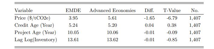
The results show that, even after matching on key characteristics, credits from EMDE remain on average $1.65 lower than those from AE ($3.95 vs $5.61 per tCO2e). Differences in credit age, project age, and inventory are minimal and statistically insignificant. This implies that the country-level price gap persists even after accounting for fundamental project characteristics, pointing to additional factors beyond observable project quality.

4.2.2 Home bias 

A potential driver of the price gap in carbon credit markets is home bias, that is the tendency of buyers to prefer credits from projects located in their own country or region. This preference may arise due to factors such as familiarity, trust, regulatory incentives, or alignment with local sustainability goals. In the context of carbon markets, home bias could lead buyers to favour domestic projects over foreign ones, even if the latter offer similar or better climate benefits. This behaviour could create price disparities and limit the efficiency of the global carbon market in directing resources toward the most cost-effective emissions reduction projects. 

To examine the potential role of investor home bias, we analyse the geographic relationship between buyers and project countries in carbon credit transactions. For this purpose, we construct a dataset at the project-month level, consistent with the main analysis, but restrict the sample to transactions with available buyer and buyer-country information. We aggregate credit prices and project characteristics at the project-month level, ensuring comparability with prior specifications. The resulting dataset includes 5,382 project-month observations. 

To address the limited availability of return data, we use the log of the raw carbon credit price as the dependent variable. This transformation also helps to stabilize fluctuations in price levels and improve the statistical properties of the regression model, potentially yielding a more stationary and well-behaved outcome variable. 

Table 10. Home Bias 

This table reports regression results testing the home bias hypothesis. The dependent variable, Log(Price)i,t, is the log-transformed price of carbon project i in month t. SameCountryi,t is the average of a dummy variable equal to one if the buyer and project are located in the same country. SameContinenti,t is the average of a dummy variable equal to one if the buyer and project are located on the same continent. Distancei,t denotes the average geographic distance (in thousand kilometers) between the capital city of the buyer country and that of the project country. All regressions are estimated at the project-month level. Standard errors are clustered at both the project and year-month levels. Statistical significance is denoted by * p < 0.10, ** p < 0.05, *** p < 0.01.

Table 10 reports the regression results assessing whether geographic proximity between buyers and project countries helps explain differences in carbon credit prices. The primary independent variable of interest, EMDEi , is a binary indicator equal to one if the credit originates from a project located in an emerging or developing economy, and zero otherwise. Model (1) serves as a baseline. Models (2) to (4) add different proxies for home bias. SameCountryi,t in Model (2) measures whether the buyer and the project are located in the same country; SameContinenti,t in Model (3) captures whether they are from the same continent; and Distancei,t in Model (4) measures the average distance between the capital cities of the buyer and project countries, in thousands of kilometers. All regressions include fixed effects for project sector, registry, and year-month. 

The results show that carbon credits from EMDEs consistently receive lower prices compared to those from advanced economies, even after accounting for project characteristics and fixed effects. In all four models, the coefficient on EMDEi remains negative and statistically significant. By contrast, the three home bias variables, SameCountryi,t, SameContinenti,t, and Distancei,t, do not display statistical significance in any specification. This suggests that buyers do not systematically prefer geographically closer projects, and proximity alone does not explain the observed pricing gap. Instead, persistent price differences are likely linked to broader concerns or market perception—factors not necessarily tied to geographic distance. 

4.2.3 Governance quality across economies 

A final potential explanation for price differences in the voluntary carbon market is the quality of governance in project host jurisdictions. Governance quality refers to the effectiveness of institutional frameworks in ensuring transparency, regulatory enforcement, and rule-based decision-making. These attributes shape how environmental standards are implemented and how credible issuance and verification processes are perceived by market participants. Buyers may be willing to pay more for credits from countries with stronger legal and regulatory institutions, which are generally associated with lower risks of fraud, underperformance, or non-compliance. 

Although voluntary carbon markets operate independently of formal government regulation, the broader institutional environment can still influence market expectations. Well-functioning legal systems and transparent administrative practices can foster trust in credit quality and delivery, supporting higher valuations. Conversely, weaker governance may prompt buyers to apply discounts due to concerns about oversight, enforcement reliability, or long-term credit validity. 

To examine this channel, we use governance indicators from the Worldwide Governance Indicators (WGI) dataset (World Bank, 2024b).³² The WGI assesses six dimensions: Voice and Accountability (VA), Political Stability and Absence of Violence (PV), Government Effectiveness (GE), Regulatory Quality (RQ), Rule of Law (RL), and Control of Corruption (CC). We focus on the four most relevant to project credibility: CC, GE, RL, and RQ, since VA and PV are less directly linked to market mechanisms or regulatory enforcement. To avoid simultaneity bias, we use lagged values of these indicators so that governance is treated as a predetermined factor rather than an outcome of market activity. Observations without WGI data are excluded. 

We also test for heterogeneous effects by interacting each governance indicator with an EMDE dummy. These interaction terms allow us to assess whether governance improvements yield similar pricing effects across country groups, or whether structural disadvantages in EMDEs dampen their impact. 

The results presented in Table 11 provide important insights into the role of governance quality indicators of jurisdictions in explaining the carbon credit price gap between advanced and emerging and developing economies. In Column (1), the baseline specification shows that credits from EMDEs are priced approximately 9% lower than those from advanced economies, with the coefficient on the EMDEi indicator being negative and statistically significant at the 1% level. Columns (2)–(5) introduce four governance indicators from the Worldwide Governance Indicators (WGI) dataset: Control of Corruption (CC), Government Effectiveness (GE), Rule of Law (RL), and Regulatory Quality (RQ), interacted with the EMDE indicator to assess heterogeneous effects. Across these models, the inclusion of governance measures significantly alters the relationship between project location and price. Notably, the coefficient on EMDEi becomes statistically insignificant in Columns (2), (4), and (5), suggesting that a substantial portion of the EMDE price discount can be attributed to differences in institutional quality. 

Among the four governance dimensions, Rule of Law (RL) exhibits the strongest and most consistent relationship with carbon credit prices. In Column (4), a one-unit increase in RL is associated with a 17% increase in log(price), which translates to approximately a 105% increase in actual credit price.³³ Moreover, the interaction term RL×EMDE is negative and statistically significant, indicating that while stronger legal institutions raise prices across all countries, the marginal benefit is significantly weaker in EMDEs. This asymmetric effect is also observed, albeit less robustly, for the Control of Corruption indicators.

Table 11. The impact of governance indicator on carbon credit price 

This table presents the regression results of carbon credit prices on the governance quality indicators of the project’s host jurisdiction. EMDEi is a binary variable equal to one if the project country is an emerging and developing economy and zero otherwise. Column (1) is benchmark model, columns (2) to (5) individually include one governance quality indicator: CCi,t−1 (Control of Corruption), GEi,t−1 (Government Effectiveness), RLi,t−1 (Rule of Law), and RQi,t−1 (Regulatory Quality). Control variables include Log(Price)i,t−1 , Credit Agei,t, Project Agei,t, CCBi (Climate, Community, and Biodiversity standards), No.SDGi (Sustainable Development Goals), Log(Inventory)i,t−1 , Turnoveri,t−1. Sector, registry, and year-month fixed effects are included in all specifications. Standard errors are clustered at the project and year-month levels. Statistical significance is denoted by * p<0.10, ** p<0.05, *** p<0.01.

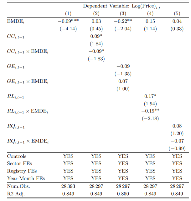
These findings suggest that buyers value credits from jurisdictions with sound legal and regulatory institutions. However, they also imply that even when EMDEs improve their governance, these improvements may not translate into equivalent pricing benefits. This asymmetry may stem from buyer scepticism, lack of market familiarity, or perceptions of enforcement risk. 

Improving governance is therefore a necessary but not sufficient condition for narrowing the price gap. Broader efforts are needed to increase transparency, build market trust, and enhance institutional visibility in emerging markets. At the country level, mechanisms such as standardized contracts, legal clarity on ownership, third-party credit ratings, and safeguards against project failure could help reinforce the credibility of credits from underrepresented regions. At the program level, ongoing initiatives such as those led by the Integrity Council for the Voluntary Carbon Market (ICVCM) aim to strengthen the integrity of crediting standards and verification frameworks. Together, national reforms and programlevel safeguards could ensure that improvements in governance are more fully reflected in carbon credit pricing. 

Taken together, the analysis in this section provides strong evidence of a persistent price gap between carbon credits from advanced economies and those from emerging market and developing economies. While differences in project quality explain part of the disparity, they do not fully account for the lower valuations of EMDE-based credits. Geographic proximity between buyers and projects, which often cited as a source of home bias, does not appear to play a meaningful role in price formation. Instead, the most influential factor is governance quality in the project host country, particularly the strength of legal institutions and regulatory effectiveness. Even so, improvements in governance in EMDEs are not always matched by equivalent pricing gains, suggesting deeper market frictions related to perception, transparency, or buyer risk appetite. These findings point to the need for structural reforms and market infrastructure enhancements to improve trust and pricing efficiency, ensuring that the voluntary carbon market delivers fairer outcomes across regions and channels capital toward the most impactful mitigation opportunities. 

5 Robustness 

In this section, we perform robustness checks to verify the reliability and consistency of our results under alternative assumptions and data filters. 

5.1 Using data from 2022 onwards

The primary analysis spans the period from 2017 to December 2024. However, it is important to note that AlliedOffsets incorporated actual market data only from 2022 onwards, while earlier years (2017–2021) involve adjusted estimates based on Ecosystem Marketplace sectoral price trends. To ensure the robustness of our results against potential inaccuracies in pre-2022 data, we restrict the analysis to the 2022–2024 period. Specifically, we run the empirical test of (1) that analysing the determination of carbon credit return. 

Table 12 presents a robustness check using data from 2022 onwards, allowing us to assess whether the relationships identified in the full sample (2017–2024, Table 4) continue to hold in the more recent period. The results broadly confirm the main patterns, but several coefficients exhibit changes in magnitude or significance, reflecting possible structural shifts in the voluntary carbon market post-2021.

The main relationships identified earlier remain intact, but several coefficients change in magnitude, indicating shifts in market dynamics post-2021. Credit age continues to exert a negative and highly significant effect on returns in all models, with a substantially larger magnitude (–0.75 to –0.79 vs. –0.42 to –0.48 in the full sample), reinforcing the view that older credits face deeper discounts in recent years, possibly due to tighter buyer standards or evolving quality benchmarks. Project age remains positive and significant, with coefficients roughly double those in the full sample, suggesting that maturity and operational track record have become even stronger pricing supports.

The mean-reversion effect in lagged returns persists across all specifications, while the impact of lagged inventory is again negative and significant, with larger coefficients than in the full period—pointing to heightened sensitivity to supply pressure. Lagged volatility (Column 4) remains positive and significant, consistent with investors requiring higher returns for projects with recent price variability.

By contrast, the pricing effects of CCB certification and SDG alignment are less stable. CCB alternates between positive and negative significance across models, and the number of SDGs is significant only in Column (2), implying that co-benefit labels have become less reliable pricing signals.

Overall, the post-2021 subsample confirms the core determinants of returns identified in the full-sample analysis—credit age, project age, inventory, and mean reversion—while revealing that some effects have strengthened. Larger absolute coefficients on credit age and inventory, coupled with greater sensitivity to volatility, suggest that the voluntary carbon market has become more discriminating and potentially more segmented in the post-2021 period, reflecting increased buyer scrutiny, policy changes, and shifting investor sentiment in a maturing market.

Table 12. Regression of carbon monthly return (2022 onwards) 

This table presents regression results based on Equation (1), using data from January 2022 onwards. The analysis evaluates whether the main relationships observed in the full sample remain consistent in the post-2021 period.

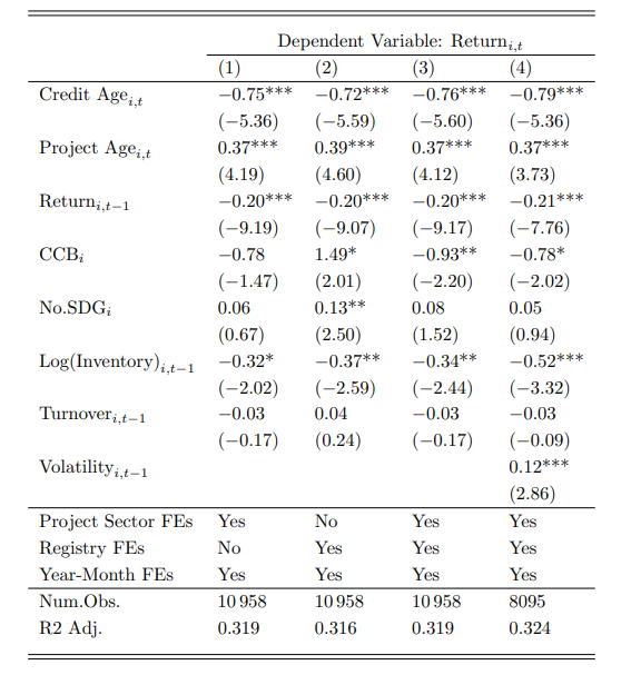
6 Conclusion 

This paper examines price discovery, price disparities, and market segmentation in the voluntary carbon market (VCM) using transaction-level data from 2017 to 2024. The analysis reveals several consistent determinants of carbon credit returns. Credit age is strongly and negatively associated with returns, indicating that older vintages are systematically discounted, whereas project age is positively associated with returns, reflecting a premium for operational track record and credibility. Market microstructure variables, such as inventory levels and lagged returns, point to persistent mean reversion and supply driven price pressure. These patterns hold across multiple model specifications and remain robust when restricting the sample to the post-2022 period, when higher-quality market data became available.

We also document a persistent and economically meaningful price gap between credits from advanced economies (AEs) and those from emerging market and developing economies (EMDEs). In the full sample, EMDE credits are priced at an average of USD 4.98 compared with USD 6.90 for AE credits. Matched-pair analysis, which controls for key observable characteristics, shows that the gap remains sizeable—around USD 1.65 per tonne—indicating that part of the disparity cannot be explained by observable quality indicators. This residual difference may reflect unpriced governance risk, buyers’ perceptions of institutional quality, or other market frictions.

Beyond jurisdictional governance, two complementary forces may also shape the price gap. First, domestic compliance carbon prices (carbon allowances or carbon taxes) can influence what firms are willing to pay for offsets. In systems where certain offsets are permitted for compliance, the prevailing policy price can serve as a loose reference point.³⁴ In our voluntary-only sample, however, any direct pass-through appears limited, and host-country credibility remains the dominant factor. Second, cross-jurisdictional heterogeneity in marginal abatement costs (MAC) may generate systematic price differences: countries with abundant low-cost mitigation opportunities tend to supply cheaper credits.³⁵ Our design already absorbs much of the technology-level cost heterogeneity through project-type controls and matched comparisons, yet within-type, jurisdiction-specific MAC variation (e.g. energy mix, land and opportunity costs, regulatory burden) may persist. Although comprehensive MAC series and compliance-price histories are not available for all jurisdictions and years in our sample window, future work could incorporate country-year proxies—such as carbon intensity, energy mix, or MAC estimates—to further disentangle these channels.

A key challenge highlighted by our findings is the absence of a standardised pricing mechanism in the voluntary carbon market. Current prices reflect a complex and opaque mix of certification methodologies, project types, and jurisdictional governance quality, leading to substantial variation and undermining comparability across credits. One possible solution is the development of a standardised pricing framework or benchmark system that adjusts for underlying project characteristics and institutional risk. In this context, independent carbon credit rating agencies—such as BeZero Carbon, Sylvera, and Calyx Global—have emerged to fill informational gaps by evaluating credit integrity. These agencies improve market transparency, facilitate more accurate valuations, and reduce information asymmetries for investors. Although platforms such as Platts, CBL, and Xpansiv already publish price benchmarks, broader adoption and comparability remain limited due to methodological differences. Wider recognition of these tools, alongside consensus on quality standards and improved access to project-level data, will be essential for achieving credible, investment-grade pricing in the VCM.

An alternative or complementary approach is to enhance credibility and buyer confidence through assurance mechanisms tailored to the voluntary carbon market, particularly for projects in emerging and developing economies. In recent years, specialised insurance products—such as those offered by Oka, The Carbon Insurance Company, and Howden—have emerged to cover risks of invalidation, reversal, or political uncertainty, thereby reducing perceived governance risk and strengthening investor confidence in EMDE-based credits.³⁶ At the same time, market-level initiatives such as the Integrity Council’s Core Carbon Principles aim to raise baseline integrity across crediting programmes. While these instruments differ in scope, they share the objective of improving transparency, reducing risk premia, and facilitating greater capital flows into high-quality projects. Together, these mechanisms represent promising steps towards narrowing the credibility gap and enabling more equitable participation of EMDEs in global carbon markets.

Footnotes: 

¹ The author would like to thank Pedro Gurrola-Perez, Owain Johnson, Simon Pabst, Paula Redondo Pereira, Victoria Powell, Bursa Carbon Exchange, and the research team of WFE for their useful comments. The views expressed in this paper are of the author and do not necessarily reflect those of the World Federation of Exchanges or its member institutions. Any errors are mine. 

² World Federation of Exchanges, [email protected] 

³ In contrast, the compliance carbon market operates under mandatory national, regional, or international carbon reduction regimes. The voluntary carbon market allows companies and individuals to purchase carbon credits on a discretionary basis, independent of regulatory obligations. 

⁴ See Financial Times (2024); IOSCO (2023b). 

⁵ Liu and Gurrola-Perez (2025) document that 73.73% of projects are developed in emerging and developing countries, collectively generating 75.13% of total carbon credits. 

⁶ See UNEP (2023). 

⁷ The transaction prices in the AlliedOffsets database are sourced from brokers, exchange partners, and project developers worldwide. 

⁸ More institutional details on CCMs can be found in IOSCO (2023a). 

⁹ Technologies that actively remove CO2 from the atmosphere are also called Carbon Dioxide Removal (CDR); see SIX Group, “Net Zero: How Does That Actually Work?,” SIX Blog. Available at: https://www.six-group.com/en/blog/carbon-removal.html. 

¹⁰ The Clean Development Mechanism (CDM), established under the Kyoto Protocol and later incorporated into Article 6.4 of the Paris Agreement, shares similarities with the VCM in that both allow for the financing of emission reduction projects in exchange for carbon credits. Under the CDM, developed countries with legally binding emission reduction targets can invest in projects in developing countries to earn Certified Emission Reductions (CERs), each representing one metric ton of CO2 reduced or avoided. However, the CDM is a compliance mechanism strictly regulated by the United Nations, whereas the VCM operates independently through private certification standards. Additionally, VCM projects can be implemented globally, while CDM projects are limited to developing countries as part of international climate cooperation. 

¹¹ For example, Xpansiv CBL introduced carbon offset spot contracts, while CME Group offers carbon futures contracts, enabling participants to trade carbon credits with greater transparency and market efficiency. Liu and Gurrola-Perez (2025) provide a list of the main platforms that trade carbon offset products. 

¹² The Voluntary Registry Offsets Database, developed by the Berkeley Carbon Trading Project, compiles data on all carbon offset projects, credit issuances, and credit retirements listed globally by the four major voluntary offset registries: Verra, Gold Standard, ACR, and CAR. Further details on project scopes and category definitions can be found at: https://gspp.berkeley.edu/assets/uploads/page/VROD-ScopesTypes.pdf. 

¹³ Gold Standard provides the ability to generate ex-ante credits, called PERs (Planned Emissions Reductions), for forestation projects. PERs represent future carbon sequestration in trees. Once the sequestration is verified through ex-post monitoring, PERs can be transitioned to VERs (Verified Emissions Reductions) and used like any ex-post credit. 

¹⁴ For this study, we use the retirement table within the database. Transactions related to Carbon Dioxide Removal (CDR) are excluded from the analysis, as these projects are typically off registries and include only 128 transactions with available pricing data. 

¹⁵ According to AlliedOffsets, retirement prices from 2022 onwards are based on actual market data, while price estimates between 2017 and 2021 rely on market trends and adjustments. 

¹⁶ The vintage year, or the duration between the credit’s vintage year and its retirement year, is a crucial determinant of credit pricing. Credits with vintage years exceeding the transaction year represent Planned Emission Reductions (PERs), reflecting future intentions to reduce emissions rather than reductions that have already occurred. 

¹⁷ To mitigate the influence of potential outliers, variables such as price, return, credit age, project age, lag return, lag return volatility, lag turnover and lag log(inventory) are winsorized at the 2.5th and 97.5th percentiles. 

¹⁸ Specifically, return is calculated as (log Pt − log Pt−k)/k, where k is the number of months between the current and most recent prior transaction, and k ≤ 3. Observations with k > 3 are excluded to ensure comparability of return estimates. 

¹⁹ This calculation requires at least six observations to ensure reliability. 

²⁰ CCB verification applies only to projects registered with Verra. 

²¹ “Revealed: more than 90% of rainforest carbon offsets by biggest certifier are worthless, analysis shows,” The Guardian, January 18, 2023. 

²² Lucien Georgeson, Jamie Saunders, Tristan Loffler, and Guy Turner, “Renewable-Energy Carbon Credits Losing Steam,” MSCI Research & Insights (blog), August 7, 2024, https://www.msci.com/research-and-insights/blog-post/ renewable-energy-carbon-credits-losing-steam. 

²³ Household device (e.g., cookstove) projects often claim a high number of SDGs because their co-benefits span many dimensions of sustainable development. They deliver direct health benefits (SDG 3) via reduced indoor air pollution, support gender equality (SDG 5) by reducing time burdens on women, alleviate poverty (SDG 1) through fuel savings, and improve energy access (SDG 7). 

²⁴ The monthly risk-free rate is sourced from the Fama and French data library. 

²⁵ That is, Turnoveri,t = (Retired Creditsi,t/Inventoryi,t−1 ) × 100. 

²⁶ At least six observations are required for a reliable volatility calculation. 

²⁷ The numerical features include Credit Agei,t, Project Agei,t, Returni,t−1, log(Inventory)i,t−1, Turnoveri,t−1, and No. SDGi. The categorical (dummy) variables include registry dummies: ACR, CAR, and GSR; project sector dummies: Agriculture, ChemProc/IndManuf, EnergyEff/FuelSwitch, Household Device, Renewable Energy, Transportation, Waste Disposal; and a dummy for CCB certification. 

²⁸ Data for the S&P 500 index and crude oil prices are obtained from Investing.com. The Climate Policy Uncertainty index is downloaded from https://www.policyuncertainty.com/climate_uncertainty.html. 

²⁹ A key reason macroeconomic variables were not included in the regression (1) is that they are project-invariant and only vary over time. Since our fixed effects specification includes year-month dummies to control for time trends, the macro variables are perfectly collinear with these fixed effects and are therefore absorbed. This prevents identification of their marginal effects in a linear fixed-effects framework. 

³⁰ Country classification follows the World Economic Outlook Database of IMF, April 2023 Edition. More information can be found at https://www.imf.org/en/Publications/WEO/weo-database/2023/April/groups-and-aggregates. 

³¹ See Abnett et al. (2024). 

³² See: https://www.worldbank.org/en/publication/worldwide-governance-indicators 

³³ This is calculated as e 0.17 − 1 ≈ 0.105. Please revise the footnote if your original elasticity was 0.72. 

³⁴ Some systems allow limited use of offsets for compliance, e.g. California (offsets capped at 4% of 2021–2025 emissions and 6% for 2026–2030). In California’s cap-and-trade system, firms may use a limited share of ARB Offset Credits (ARBOCs)—compliance offsets issued by CARB under its own protocols—as part of compliance; these differ from voluntary credits, though some legacy voluntary credits were converted into ARBOCs under the Early Action process. By contrast, the EU ETS (post-2020) and the UK ETS do not allow offsets for compliance. 

³⁵ IMF research (Black et al. (2023)) shows that abatement costs are generally higher in high-income countries and lower in low- and lower-middle-income countries, reflecting differences in mitigation opportunities—consistent with cross-country MAC heterogeneity 

³⁶ “Oka launches green credit insurance offering,” Reinsurance News, 21 August 2025. “Howden creates warranty and indemnity policy for carbon credits,” Reuters, 21 June 2024.

References

Abnett, K., V. Volcovici, and K. Strohecker (2024, November). Developing nations blast $300 billion COP29 climate deal as insufficient. Reuters. Available at: Reuters.

Bartram, S. M., K. Hou, and S. Kim (2022). Real effects of climate policy: Financial constraints and spillovers. Journal of Financial Economics 143, 668–696. Available at: https://doi.org/10.1016/ j.jfineco.2021.06.015.

Black, S., I. W. H. Parry, V. Mylonas, N. Vernon, and K. Zhunussova (2023, June). The imf-world bank climate policy assessment tool (cpat): A model to help countries mitigate climate change. IMF Working Paper 2023/128, International Monetary Fund.

BloombergNEF (2024, January 10). Carbon offset demand hits record in 2023 off huge december. Available at: Bloomberg.

Bolton, P. and M. Kacperczyk (2023). Global pricing of carbon-transition risk. The Journal of Finance 78 (6), 3677–3754.

Bolton, P., A. Lam, and M. Muˆuls (2023). Do carbon prices affect stock prices? Available at SSRN . Available at: https://ssrn.com/abstract=4369925.

Borri, N., Y. Liu, A. Tsyvinski, and X. Wu (2024, August). Inefficiencies of carbon trading markets. SSRN Electronic Journal. Available at: https://ssrn.com/abstract=4923646.

Bustamante, M. C. and F. Zucchi (2024, January). Dynamic carbon emission management. (2024/2885). Available at SSRN: https://ssrn.com/abstract=4691167 or http://dx.doi.org/10.2139/ssrn.4691167.

Cludius, J., H. Galster, S. Healy, V. Noka, and L. Lam (2022, December). The role of financial operators in the ETS market and the incidence of their activities in determining the allowances’ price. Technical Report PE 740.052, European Parliament. Available at: https://www.europarl.europa.eu/ thinktank/en/document/IPOL_STU(2022)740052.

Esenduran, G., H. S. Heese, and G. Souza (2024). Getting to the green: Should a profit-maximizing firm buy carbon offsets or invite consumers to buy them? Available at: https://ssrn.com/abstract= 4975444 or http://dx.doi.org/10.2139/ssrn.4975444.

ESMA (2022). Emission allowances and associated derivatives - final report. Technical report, European Securities and Markets Authority (ESMA). Available at: https: //www.esma.europa.eu/sites/default/files/library/esma70-445-38_final_report_on_ emission_allowances_and_associated_derivatives.pdf.

Financial Times (2024, September). The fragmentation of carbon markets must be fixed. Financial Times. Accessed: 2024-09-11. Available at: https://www.ft.com/content/ 70cc3e67-30c8-42b1-8012-51b496816e63.

Forest Trends’ Ecosystem Marketplace (2023). State of the Voluntary Carbon Market 2023. Washington, DC: Forest Trends Association. Available at: https://www.ecosystemmarketplace.com/ publications/state-of-the-voluntary-carbon-market-report-2023/.

Forest Trends’ Ecosystem Marketplace (2024). State of the Voluntary Carbon Market 2024. Washington, DC: Forest Trends Association. Available at: https://www.forest-trends.org/publications/ state-of-the-voluntary-carbon-market-2024/. 

Green, J. F. (2021). Does carbon pricing reduce emissions? a review of ex-post analyses. Environmental Research Letters 16 (4), 043004. Available at: https://doi.org/10.1088/1748-9326/abdae9.

Gu, S., B. Kelly, and D. Xiu (2020). Empirical asset pricing via machine learning. The Review of Financial Studies 33 (5), 2223–2273. Available at: https://doi.org/10.1093/rfs/hhaa009.

IOSCO (2023a, July). Compliance carbon markets. Available at: https://www.iosco.org/library/ pubdocs/pdf/IOSCOPD740.pdf.

IOSCO (2023b, December). Voluntary carbon markets, consultation report. Available at: https://www.iosco.org/library/pubdocs/pdf/IOSCOPD774.pdf.

Jarmuzek, M. and T. Lybek (2018). Can Good Governance Lower Financial Intermediation Costs? IMF Working Papers 18 (279), 1.

Ke, G., Q. Meng, T. Finley, T. Wang, W. Chen, W. Ma, Q. Ye, and T.-Y. Liu (2017). LightGBM: A highly efficient gradient boosting decision tree. In Advances in Neural Information Processing Systems, Volume 30.

Kim, S., T. Li, and Y. Wu (2024). Carbon offsets: Decarbonization or transition-washing? Available at: https://ssrn.com/abstract=4762799 or http://dx.doi.org/10.2139/ssrn.4762799.

Liu, Y. and P. Gurrola-Perez (2025). The dynamics of global voluntary carbon markets: An empirical analysis of the carbon credits lifecycle. WFE Working Paper, available at: https://www.world-exchanges.org/our-work/articles/ dynamics-voluntary-carbon-markets-empirical-analysis-carbon-credits-lifecycle.

Pedersen, L. H. (2023). Carbon pricing versus green finance. Available at: https://ssrn.com/abstract=4382360 or http://dx.doi.org/10.2139/ssrn.4382360.

Quemin, S. and M. Pahle (2023). Financials threaten to undermine the functioning of emissions markets. Nature Climate Change 13, 22–31.

Twidale, S. (2024, February). Global carbon markets value hit record $949 bln last year - LSEG. Reuters. Available at: Reuters.

UNEP (2023). Adaptation gap report 2023: Underfinanced. underprepared. inadequate investment and planning on climate adaptation leaves world exposed. Available at: https://doi.org/10.59117/20. 500.11822/43796.

Wetterberg, K., E. Lanzi, and N. G´omez (2025). Exploring governments’ efforts to shape carbon credit markets: Possible actions to enhance integrity. OECD Environment Working Papers 263, OECD Publishing, Paris.

World Bank (2023). State and trends of carbon pricing 2023. Available at: https://carbonpricingdashboard.worldbank.org/.

World Bank (2024a). State and trends of carbon pricing 2024. Available at: http://hdl.handle.net/10986/41544.

World Bank (2024b). Worldwide governance indicators, 2024 update. Accessed on 10/30/2024. Available at: http://www.govindicators.org.

Yadav, K. (2024, January 9). Vcm sees bumper retirements in December with 2.6 times rise on month. Available at: S&P Global Commodity Insights 

Appendix

A Price Distribution of Carbon Credits by Project Sector

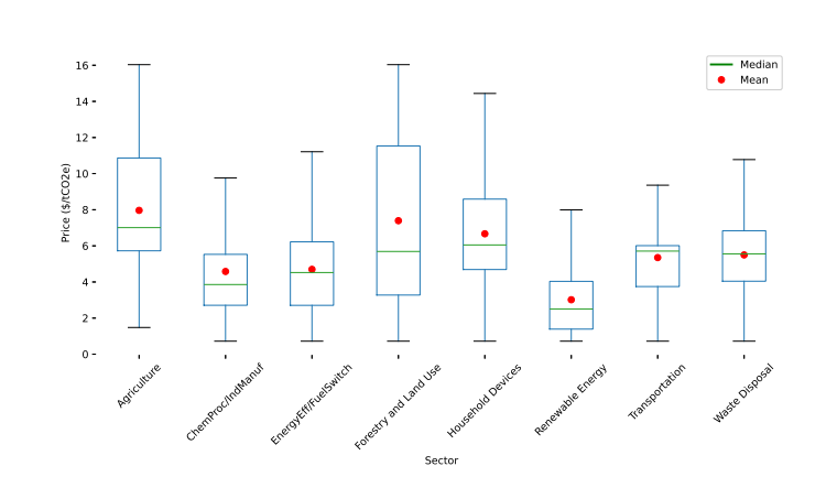
Figure A1. Price Distribution of Carbon Credits by Project Sector This figure plots the price distribution of carbon credits grouped by project sector. Each box represents the interquartile range (IQR), with whiskers extending to show the range of the data, excluding outliers. The green horizontal line within each box represents the median price for that sector, while the red dots indicate the mean price.

B Multivariate Analysis with Project Sector and Registry dummy 

Table A1. Multivariate Analysis Results This table reports the regression results for Equation (1). Column (1) includes registry dummies, with Verra omitted as the baseline category. Column (2) includes project sector dummies, with Forestry and Land Use omitted as the baseline category. ChemProc/IndManuf refers to Chemical Process/Industrial Manufacuring, EnergyEff/FuelSwitch refers to Energy Efficiency/Fuel Switching. Statistical significance is denoted by * p<0.10, ** p<0.05 , *** p<0.01.

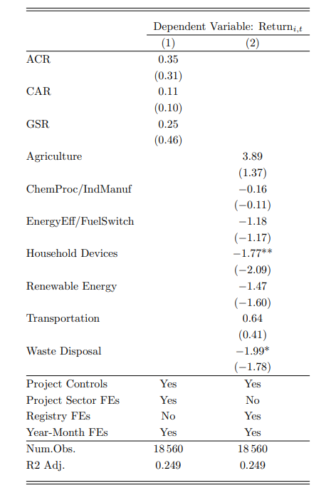
C Trading Volume of Carbon Offset Futures

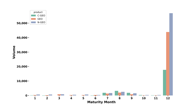
Figure A2. Aggregate Trading Volume of Carbon Offset Futures by Contract Maturity Month This figure presents the average aggregate trading volume of carbon offset futures categorized by their maturity month. The analysis considers trading volumes within the one-year period preceding each contract’s maturity. The sample period spans from March 2021 to December 2023 and includes futures contracts maturing between February 2022 and December 2023. For each futures contract, the aggregate trading volume is calculated over the year prior to its maturity. Subsequently, the average volume is computed across contracts with the same maturity month.